
Lastkollektive in der FVA-Workbench
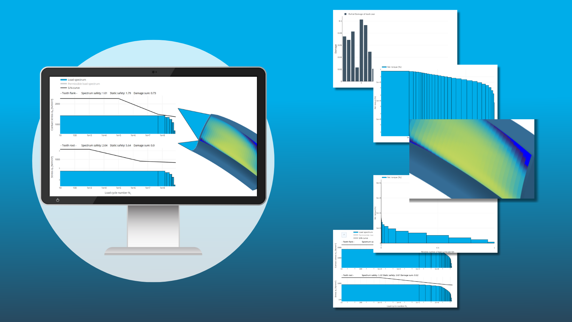
Bild: © FVA GmbH
Realistische Modellierung von Lasten: Die Rolle von Lastkollektiven
Bei der Konstruktion und Validierung mechanischer Systeme, insbesondere bei komplexen Anwendungen im Antriebsstrang, stehen Ingenieure vor der Herausforderung, Betriebslasten möglichst genau zu berücksichtigen. In der Regel stützen sich gängige Konstruktionsmethoden auf Nenn-, statische oder Extremlastfälle, um die Sicherheit der Bauteile zu gewährleisten. Diese Ansätze bieten zwar eine solide Grundlage, führen jedoch häufig zu übermäßig konservativen Konstruktionen, erhöhtem Materialverbrauch und eingeschränkten Einblicken in das tatsächliche Verhalten der Bauteile unter realistischen Bedingungen.
Lastkollektive bieten eine ausgefeiltere Alternative, indem sie die Häufigkeit und Größe der im Betrieb auftretenden unterschiedlichen Lasten statistisch beschreiben. So ermöglichen sie ermüdungsgerechte Konstruktionen, verlässliche Lebensdauerprognosen, die optimale Auslegung für verschiedene Lastfälle sowie die Berechnung der Zuverlässigkeit ganzer Antriebsstränge. Gerade bei modernen Anwendungen wie Elektroantrieben mit hochdynamischen Lastprofilen ist dieser Detailgrad nicht nur vorteilhaft, sondern unerlässlich.
Die Relevanz von Lastkollektiven zeigt sich auch in zahlreichen technischen Normen und Richtlinien, darunter ISO 281 [1] und ISO 16281 [2] für Wälzlager, ISO 6336 [3] für Stirnräder, ISO 10300 [4] für Kegelräder und die FKM-Richtlinie [5] als universell einsetzbarer Ansatz. All diese Normen basieren auf Methoden wie dem Rainflow-Zählalgorithmus [6] und der Palmgren-Miner-Regel. Diese Methoden bilden das Rückgrat der zuverlässigkeitsbasierten Konstruktionen, die in regulierten oder sicherheitskritischen Branchen zunehmend gefordert werden.
Trotz ihrer Vorteile sind Lastkollektive in der Industrie noch nicht flächendeckend verbreitet. Gründe dafür sind unter anderem die vermeintliche Komplexität ihrer Integration in Entwicklungsprozesse, Unsicherheiten bei den Lastannahmen sowie mangelnde Software-Unterstützung. Die FVA-Workbench schließt diese Lücke mit einer speziell für die Analyse mechanischer Antriebssysteme entwickelte Simulationsplattform, die Lastkollektiv-Bewertungen vollständig unterstützt.
Dieses White Paper stellt zunächst das Prinzip der Lastkollektive vor, erläutert ihre praktische Bedeutung und zeigt, wie sie in der FVA-Workbench angewendet werden können. Es richtet sich an Ingenieure, die ihr Wissen über Tragfähigkeitsberechnungen vertiefen möchten, sowie an Entscheidungsträger, die den strategischen Nutzen realistischer Lastbewertungen besser verstehen wollen.
Vorteile von Lastkollektiven gegenüber Nennlasten aus technischer Sicht
Reale Betriebsbedingungen sind selten durch gleichmäßige, stationäre Lasten gekennzeichnet. Stattdessen schwanken sie aufgrund externer Faktoren wie Umgebung, Nutzungsverhalten und Systemdynamik. Beispiele hierfür sind:
Elektrofahrzeuge: Schnelle Drehmomentänderungen durch Beschleunigung, Bremsen und Rekuperation
Industriegetriebe: Lastschwankungen über Arbeitszyklen oder Produktionsschichten hinweg
Windkraftanlagen: Ständige Schwankungen durch wechselnde Windgeschwindigkeiten
Konstruktionen, die nur auf Nennlasten basieren, führen oft zu überdimensionierten Bauteilen, um seltene Extremfälle abzudecken. Dies sorgt zwar für Sicherheit, führt jedoch zu ineffizientem Materialeinsatz, höherem Gewicht und steigenden Kosten. Zudem liefern sie keine verlässlichen Aussagen zur tatsächlichen Lebensdauer oder zum Ausfallrisiko.
Zudem ermöglichen nominale Auslegungsansätze keine ermüdungsbasierende Lebensdauerprognose. Sie beantworten lediglich die Frage: „Hält das Bauteil den schlimmsten Fall aus?“, nicht jedoch „Wie lange hält es unter realen Einsatzbedingungen?“ oder „Wie hoch ist die Ausfallwahrscheinlichkeit innerhalb der Garantiezeit?“. Hier kommt das Konzept der Lastkollektive ins Spiel.
Ein Lastkollektiv (manchmal auch Lastspektrum genannt) ist eine komprimierte statistische Darstellung der unterschiedlichen mechanischen Belastungen, die im Laufe der Zeit auftreten. Statt eines einzelnen Nennlastwertes beschreibt es die Häufigkeit und Höhe zahlreicher Lastfälle, meist in Form diskreter Laststufen mit den dazugehörigen Lastwechselzahlen oder Lastdauern. Dies ist besonders wichtig für die Analyse der Beanspruchbarkeit von Bauteilen und Systemen, die dynamischen, nicht-stationären oder variierenden stationären Betriebsbedingungen ausgesetzt sind.
Im Kern beantwortet ein Lastkollektiv zwei Fragen:
Wie hoch war die Belastung? (z. B. Drehmomentniveau, Kraftamplitude)
Wie oft ist diese Belastung aufgetreten? (z. B. Anzahl der Lastwechsel oder Betriebszeit innerhalb eines bestimmten Lastbereichs)
Lastkollektive können je nach Anwendung und Datenquelle unterschiedliche Formen annehmen.
Zeitreihen: Belastungssignale im Zeitverlauf, die mittels Zählverfahren in Kollektive umgewandelt werden können
Histogrammbasierte Kollektive: Diskrete Fälle, die Lastniveau und Häufigkeit darstellen
Rainflow-Matrizen: Zweidimensionale Darstellungen, die häufig in der Betriebsfestigkeitsrechnung verwendet werden und aus dem Rainflow-Zählalgorithmus abgeleitet sind.
Jedes Format bietet spezifische Vorteile in Bezug auf Genauigkeit, Recheneffizienz oder Kompatibilität mit bestimmten Berechnungsmethoden.
In der Antriebstechnik sind Lastkollektive besonders wichtig für:
Vorhersage der Lebensdauer von Zahnrädern, Wellen, Lagern und anderen rotierenden sowie nicht rotierenden Teilen
Optimierung der Geometrie und Flankenmodifikationen unter verschiedenen Lastszenarien
Bewertung der Systemzuverlässigkeit, Ausfallwahrscheinlichkeit und erwarteten Lebensdauer
Vermeidung von Überdimensionierung durch den Ersatz von Worst-Case-Annahmen mit datengestützten Erkenntnissen
Umwandlung von Zeitsignalen in Lastkollektive
In vielen Entwicklungsprozessen bilden Zeitsignale die Grundlage für die Erstellung von Lastkollektiven. Dabei handelt es sich um Mess- oder Simulationsdaten von Kräften, Drehmomenten oder Beschleunigungen, die über einen bestimmten Zeitraum gemessen oder simuliert wurden. Diese Zeitreihen spiegeln das dynamische Verhalten eines Systems unter bestimmten Betriebsbedingungen wider, wie z. B. während eines Fahrzyklus, eines Testszenarios oder eines realen Nutzungsmusters.
Die Umwandlung dieser Rohdaten in ein nutzbares Lastkollektiv erfolgt in mehreren Schritten:
Schritt 1: Zeitsignal vorbereiten
Bevor ein Zählverfahren angewendet wird, muss das Zeitsignal vorbereitet werden:
Filtern: Entfernen von irrelevanten hochfrequenten Störsignalen oder nicht schädigungsrelevanten Schwingungen
Normalisierung: Anpassen der Werte an einheitliche Einheiten oder Referenzwerte
Segmentierung: Aufteilen der Signale in verschiedene Betriebsmodi, falls erforderlich
Trunkierung: Ausschließen von Start-/Stopp- oder Leerlaufphasen, die die Statistiken verfälschen
Schritt 2: Zählverfahren anwenden
Nachdem das Zeitsignal verarbeitet wurde, werden im nächsten Schritt Lastzyklen identifiziert. Das heißt, wiederholte Belastungs- oder Beanspruchungswechsel, die zur Materialermüdung beitragen. Dieser Schritt ist zentral für die Erstellung eines aussagekräftigen Lastkollektivs.
Die am häufigsten verwendete Methode ist die Rainflow-Zählung. Dabei wird eine komplexe, unregelmäßige Beanspruchungsfolge in einzelne, geschlossene Schwingspiele zerlegt. Die Rainflow-Zählung basiert auf einer werkstoffmechanischen Grundlage und kann als Algorithmus interpretiert werden, der nach geschlossenen Spannungs-Dehnungs-Hysteresen sucht (siehe Abbildung 1).
Der Flächeninhalt der Hysteresen kann als schadensrelevantes Energieäquivalent interpretiert werden. Das Ergebnis der Rainflow-Zählmethode ist die sogenannte Rainflow-Matrix, die entweder die oberen und unteren Umkehrpunkte oder die Mittel- und Amplitudenwerte aller auftretenden Hysteresen enthält.
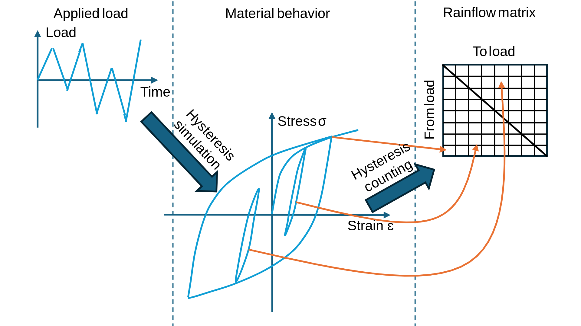
Abbildung 1: Der Rainflow-Zählalgorithmus basiert auf einer Hysterese-Simulation des realen elastisch-plastischen Materialverhaltens. Der (erweiterte) Rainflow-Algorithmus wandelt die aufgebrachten Lasten in eine Spannungs-Dehnungs-Reihe um und zählt die darin enthaltenen geschlossenen Hysteresen. Die meisten verwendeten Rainflow-Algorithmen basieren auf diesem Algorithmus, weisen jedoch durch diverse Optimierungen eine verbesserte Leistung auf.
Schritt 3: Lastkollektiv erstellen
Nach der Zählung werden die identifizierten Schwingspiele entweder direkt in Form einer Rainflow-Matrix verarbeitet oder in ein Histogramm umgewandelt. Das resultierende Kollektiv kann anschließend auf eine bestimmte Gesamtbetriebsstundenzahl oder ein definiertes Lebenszeitziel (z. B. 100.000 km, 10.000 h, 1 Million Lastwechsel) skaliert werden.
Die Umwandlung eines Zeitsignals in ein Lastkollektiv ermöglicht nicht nur die Bewertung einer einzelnen spezifischen Konstruktionsvariante. Sorgfältig aufbereitete Kollektive lassen sich, insbesondere bei klarer Trennung in Betriebsmodi und entsprechender Normalisierung, auch auf verschiedene Varianten übertragen.
Anwendungen in der Getriebe- und Antriebstechnik
Der Antriebsstrang besteht aus einer Vielzahl miteinander interagierender Komponenten wie Zahnrädern, Wellen, Lagern und Kupplungen, die während ihrer gesamten Lebensdauer komplexen, zeitlich variierenden Belastungen ausgesetzt sind. Zur Berechnung der Belastbarkeit dieser einzelnen Komponenten kann man zwar die Lastkollektive auf Bauteilebene anwenden, ohne dabei Wechselwirkungen zu berücksichtigen. Erst durch die Anwendung von Lastkollektiven auf Systemebene ermöglicht jedoch eine ganzheitliche Optimierung des gesamten Getriebes, z. B. die NVH-Optimierung mehrerer Zahnräder.
Anwendungen auf Bauteilebene
Zahnräder
Ermüdungsbewertung anhand von Wöhlerlinien und Sicherheitsfaktoren (z. B. gemäß ISO 6336)
Optimierung der Mikrogeometrie (z. B. Kopfrücknahme, Balligkeit) unter unterschiedlichen Belastungsbedingungen
Wellen
Berechnung der schadensäquivalenten Nominalbelastung (z. B. für Bauteiltests)
Ermüdungsbewertung anhand von S-N-Kurven und Sicherheitsfaktoren (z. B. gemäß FKM-Richtlinie)
Identifizierung kritischer Lastbereiche, die die Ermüdungslebensdauer beeinflussen
Lager
Berechnung der Lagerlebensdauer unter variablen Belastungen (z. B. ISO 281)
Vermeidung von Unter- oder Überschätzung der Lagerlebensdauer durch Berücksichtigung realer Lastschwankungen
Anwendungen auf Systemebene
Auslegung für mehrere Lastfälle (z. B. Optimierung von Flankenmodifikationen unter Berücksichtigung aller auftretenden Laststufen anstelle einer rein nominalen Bemessungsskala)
Berechnung der Lebensdauer und Zuverlässigkeit des Gesamtsystems unter Berücksichtigung der Wechselwirkungen zwischen den Komponenten
Dies ist für die Zuverlässigkeitsplanung, Garantiestrategien und vorausschauende Wartung von entscheidender Bedeutung.
Erstellen und Organisieren von Lastkollektiven in der FVA-Workbench
Die FVA-Workbench ist eine umfassende Simulations- und Berechnungsplattform zur Analyse, Auslegung und Optimierung mechanischer Antriebssysteme. Ein wesentliches Alleinstellungsmerkmal der FVA-Workbench ist ihre duale Basis: Die Software vereint die vollständige Unterstützung etablierter Industriestandards mit den neuesten Forschungsergebnissen aus der industriellen Gemeinschaftsforschung der Forschungsvereinigung Antriebstechnik e.V. (FVA e.V.).
Die besondere Stärke der FVA-Workbench liegt darin, dass diese forschungsbasierten Methoden nicht in versteckten Expertenmodi oder akademischen Zusatzmodulen untergebracht sind. Stattdessen stehen sie als standardisierte Berechnungsverfahren zur Verfügung: klar dokumentiert, nahtlos in den Workflow integriert und durch eine intuitive Benutzerführung leicht zugänglich.
So profitieren Ingenieure von den modernsten Berechnungsmethoden, ohne selbst Forschungsspezialisten sein zu müssen. Die Komplexität bleibt im Hintergrund, während die Anwendung übersichtlich, praxisnah und für den Konstruktionsalltag geeignet bleibt.
Arbeiten mit Lastkollektiven in der FVA-Workbench
Grundlage jeder lastkollektivbasierte Bewertung in der FVA-Workbench sind repräsentative Lastdaten. Die Software bietet dafür eine breite Palette von Methoden, um Lastsignale in Lastkollektive umzuwandeln, darunter:
Mehrparametrische Verweildauer-Zählung
Einparametrische Verweildauer-Zählung
Synthetische Lastkollektive
Standardisierte Lastkollektive
Rainflow-Zählung
Diese Prozesse werden in einer geführten Benutzeroberfläche abgebildet, die passende Standardeinstellungen je nach Anwendungskontext bereitgestellt (siehe Abbildung 2).
Die erzeugten Lastkollektive lassen sich anschließend in die lokale Projektdatenbank importieren.
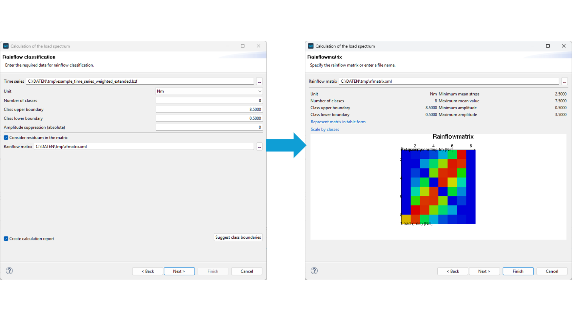
Abbildung 2: Bei der Umwandlung an Lastdaten (Zeitreihen, Kollektiven etc.) führt ein Assistent den Benutzer durch den Prozess – hier dargestellt am Beispiel der Rainflow-Zählung.
Anwendung von Lastkollektiven in der Systemberechnung
Sobald ein Lastkollektiv in der FVA-Workbench erstellt wurde, kann es direkt für Systemberechnungen verwendet werden. Die FVA-Workbench bietet zwei Berechnungsmodi für Lastkollektive: das skalierte und das flexible Lastkollektiv. Das skalierte Lastkollektiv ähnelt klassischen histogrammbasierten Lastkollektiven. Jeder Lastfall basiert auf einem Nennlastfall und wird über Skalierungsfaktoren (z. B. Drehzahl und aufgebrachtes Drehmoment) angepasst. Andererseits ermöglicht das flexible Lastkollektiv jede Kombination von Lasten, Drehzahlen und ausgewählten Gängen. Die aktiven Gänge können sich dabei je nach Lastfall unterscheiden. So lassen sich vollständig unabhängige Lastfälle anlegen und für jeden eine separate Gesamtsystemberechnung durchführen. Dadurch kann der Anwender die Auswirkungen einzelner Betriebszustände isoliert bewerten, so als wären alle Lastfälle eigenständige Nennlastfälle. Dies ermöglicht erweiterte Optimierungs- und Nachbearbeitungsmöglichkeiten, insbesondere unter Verwendung der Skriptumgebung der FVA-Workbench.
Berechnungsmethoden und unterstützte Komponenten
Die folgenden Berechnungen unterstützen die kollektivbasierte Berechnung in der FVA-Workbench:
ISO 6336 für Stirnräder
Zahnradanregung nach FVA 338 I für Stirnräder
ISO 10300 für Kegelräder
Lokale Schadensakkumulation für Kegelräder nach FVA 586 I
Ermüdungsberechnung von Wellen und Kerben unter Verwendung der FKM-Richtlinie
ISO 281 und 16281 für Wälzlager
Bei allen Berechnungen werden Lastwechsel und deren Schadensbeitrag kumulativ berücksichtigt – unabhängig davon, ob der skalierte oder der flexible Lastkollektivmodus verwendet wird. So ist eine realistische Lebensdauerprognose auf Komponentenebene unter repräsentativen Einsatzbedingungen möglich.
Visualisierung und Interpretation der Ergebnisse
Nach der Berechnung eines Lastkollektivs stellt die FVA-Workbench zahlreiche Visualisierungs- und Analysewerkzeuge bereit, die Ingenieure helfen, die Auswirkungen unterschiedlicher Belastungen auf die Bauteillebensdauer besser verstehen können.
Eine der häufigsten Visualisierungen in der Lastkollektivanalyse ist die Wöhlerlinie mit dem entsprechenden Spannungskollektiv (siehe Abbildung 3). In der FVA-Workbench werden dabei stets zwei Sicherheitsfaktoren berechnet: der statische Sicherheitsfaktor, der das Verhältnis der maximalen Last im Lastkollektiv zur statischen Grenze der Wöhlerlinie angibt, sowie die Kollektivsicherheit, die angibt, um welchen Faktor das gesamte Kollektiv skaliert werden kann, damit die Schadenssumme
unter 1 bleibt.
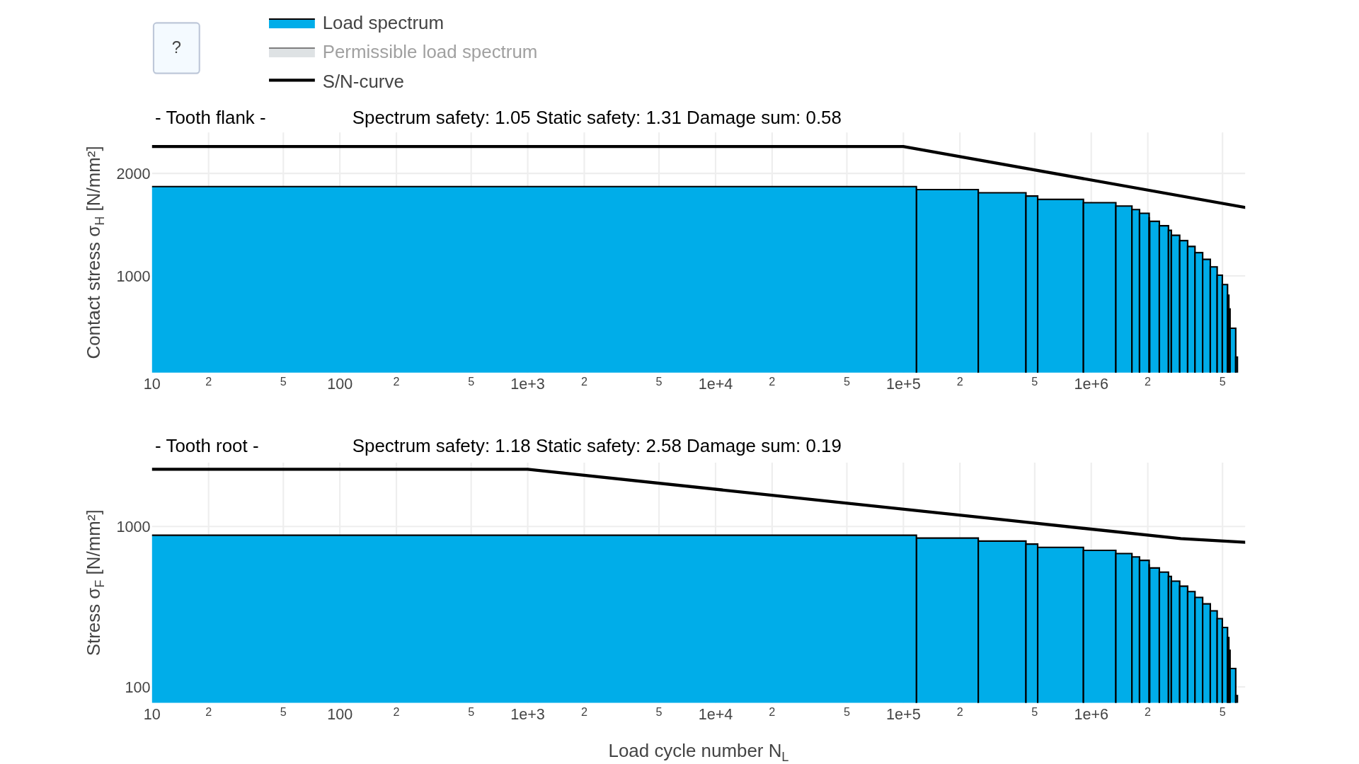
Abbildung 3: Lastkollektiv und Wöhlerlinie für Zahnflanke und Zahnfuß gemäß ISO 6336
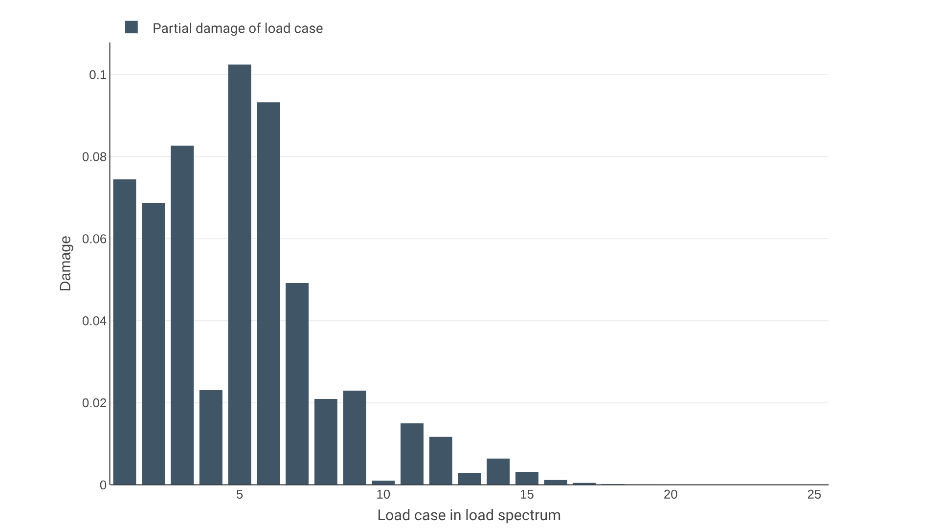
Abbildung 4: Teilschädigung der Lastfälle im Lastkollektiv zur Ermittlung des am meisten schädigenden Lastfalls
Die Teilschädigungen der einzelnen Lastfälle können ebenfalls dargestellt werden (siehe Abbildung 4). Dies hilft dabei, die Verzahnung für die Lastfälle zu optimieren, bei denen die größte Schädigung auftritt.
Die Software berechnet und zeigt Lebensdauerkennzahlen basierend auf den kumulierten Schädigungsanteilen über alle Lastzyklen hinweg an. Je nach Berechnungsmethode und Einstellungen umfassen die Ergebnisse unter anderem:
Geschätzte Lebensdauer (z. B. in Stunden, Kilometern oder Lastzyklen)
Schadenssumme (z. B. Miner-D-Wert)
Auslastungsgrad/Sicherheitsfaktor (z. B. wie nah das Bauteil an seiner Ermüdungsgrenze betrieben wird)
Da die FVA-Workbench parametrische Studien und Optimierungen unterstützt, können Anwender die Ergebnisse verschiedener Konstruktionsvarianten oder Lastszenarien vergleichen. Abbildung 5 zeigt ein Beispiel mit zwei Flankenmodifikationen, die auf dasselbe Lastkollektiv angewendet wurden. Die Flankenmodifikation auf der linken Seite ist für den Nennlastfall optimiert, während die rechte Flankenmodifikation für das gesamte Lastkollektiv optimiert ist. Die resultierende Lebensdauer der Zahnflankentragfähigkeit unterscheidet sich dabei um bis zu ca. 10 %. Dies verdeutlicht, dass das Vernachlässigen des Lastkollektivs bei der Flankenoptimierung im schlimmsten Fall die Tragfähigkeit des Zahnrads deutlich verringern kann.
Für eine detaillierte Analyse bietet die FVA-Workbench Vergleichstabellen sowie erweiterte Auswertungsfunktionen, die über die integrierte Skriptumgebung genutzt werden können, um systematische technische Entscheidungen zu unterstützen.
Alle Ergebnisse können:
als Tabellen, Bilder oder Rohdaten exportiert werden
in das automatisierte Berichtssystem (HTML und PDF) integriert werden
mit Projektmetadaten und Berechnungseinstellungen versehen werden
zur Rückverfolgbarkeit und Zertifizierung versioniert und archiviert werden
Dadurch wird sichergestellt, dass kollektivbasierte Bewertungen nahtlos in bestehende Dokumentations- und Prüfprozesse integriert werden können, sowohl für interne Zwicke als auch für Kunden oder behördliche Einreichungen.
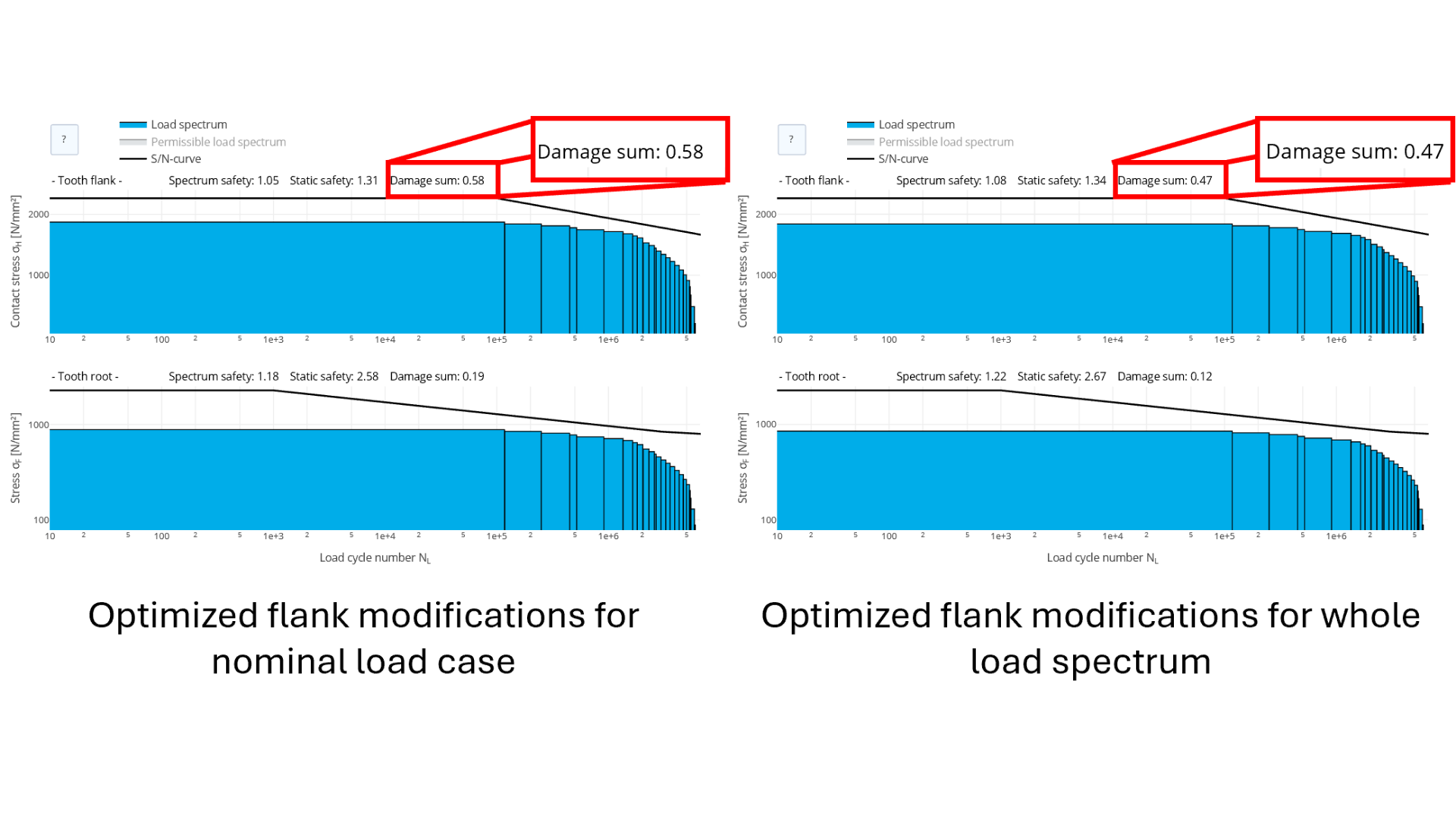
Abbildung 5: Resultierende Schadenssummen einer Stirnradstufe bei Optimierung für die Nennlast (links) und für das Lastkollektiv (rechts) – die Schadenssumme kann durch Berücksichtigung des Lastkollektivs anstelle der Nennlast deutlich gesenkt werden.
Integration von Lastkollektiven in automatisierte Arbeitsabläufe
In der Ingenieurpraxis sind Wiederholbarkeit und Effizienz ebenso wichtig wie fachliche Genauigkeit. Besonders in Unternehmen, die mehrere Produktvarianten entwickeln oder in großen Teams arbeiten, müssen Lastkollektive reproduzierbar, transparent und automatisiert handhabbar sein.
Die FVA-Workbench wurde unter Berücksichtigung dieser Anforderungen entwickelt. Ihr Ansatz zur Integration von Lastkollektiven geht weit über eine einmalige Anwendung hinaus – sie bietet ein Framework für systematisches, skalierbares Engineering.
Ingenieure können Lastkollektivvorlagen auf Basis typischer Betriebsprofile definieren, z. B.:
Standardisierte Betriebszyklen
Kundenspezifische Nutzungsdaten
Interne Lastdefinitionen aus früheren Projekten
Diese Vorlagen können gespeichert, angepasst und system- und projektübergreifend wiederverwendet werden. So wird eine einheitliche Bewertung sichergestellt und die Einrichtungszeit für wiederkehrende Arbeitsabläufe deutlich reduziert.
Da FVA-Workbench-Modelle vollständig parametrisch aufgebaut sind, können Konstruktionsvarianten mit unterschiedlichen Geometrien, Werkstoffen oder Lastbedingungen automatisiert generiert und berechnet werden. In Kombination mit der Lastkollektivauswertung ermöglicht dies:
Batch-Simulationen, bei denen mehrere Konstruktionsvarianten unter identischen Lastkollektiven bewertet werden
Automatisierte Vergleiche von Lebensdauer, Schädigung und Sicherheitsfaktoren
Optimierungsstudien zur Steigerung der Lebensdauer oder Reduzierung von Überdimensionierung
Anwendungsbeispiel
Der in Abbildung 6 dargestellte Anwendungsfall veranschaulicht, wie Lastkollektive in der FVA-Workbench als Teil eines realistischen Getriebeentwicklungsszenarios verwendet werden können.
Das Beispiel basiert auf einer Kugelmühle aus einem Kalkwerk. Die zugrunde liegenden Daten stammen aus dem FVA-Projekt 48 I [7]. Die Kugelmühle dient zum Feinmahlen von Branntkalk. Im Fokus steht hier das einstufige Untersetzungsgetriebe, das während des Mahlvorgangs unterschiedlichen Drehmomenten und Belastungen ausgesetzt ist. Die wichtigsten technischen Details des Getriebes und des Antriebsstrangs sind in Tabelle 1 zusammengefasst.
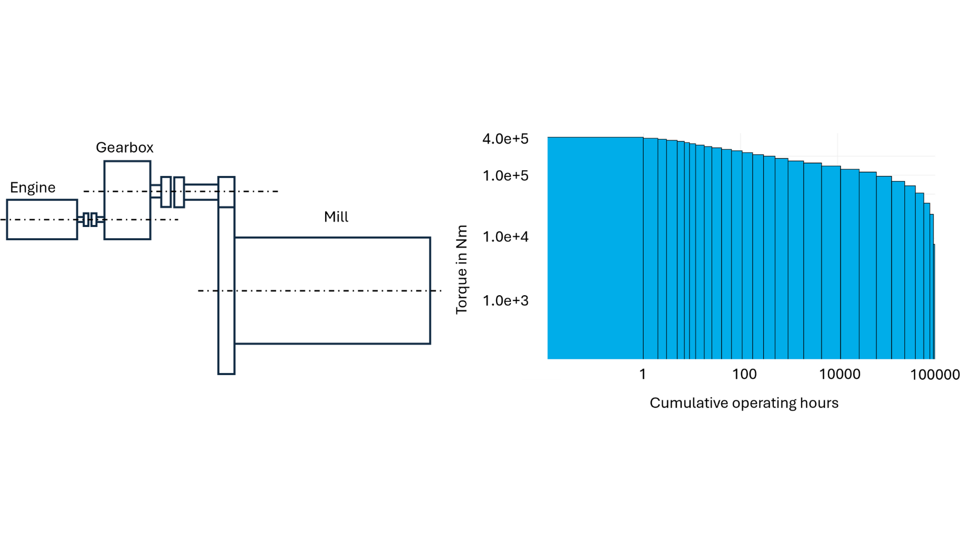
Abbildung 6: Anwendungsbeispiel – Mühle (links) und aufgebrachtes Drehmomentspektrum am Getriebeeingang (rechts)
| Eingangsdrehzahl | 985 min-1 |
| Übersetzungsverhältnis des Getriebes | 6,54 |
| Zähnezahl des Ritzels | 26 |
| Zähnezahl des Rades | 170 |
| Übersetzungsverhältnis des Kettenradgetriebes | 6,96 |
| Zähnezahl des Kettenradritzels | 23 |
| Zähnezahl des Kettenradrades | 160 |
| Drehzahl der Mahltrommel | 21,6 min-1 |
Das Getriebe der Mühle soll für eine Lebensdauer von 100.000 Stunden ausgelegt werden. In diesem Beispiel wird die resultierende Lebensdauer der Stirnradverzahnung gemäß ISO 6336, der Wälzlager gemäß ISO 281 und ISO 16281 sowie der Auslastungsgrad der Wellenkerben gemäß der FKM-Richtlinie betrachtet. Ziel ist es, das Einsparpotenzial für die einzelnen Komponenten sowie für das Gesamtsystem aufzuzeigen, das sich durch die Verwendung von Lastkollektiven anstelle der Nennlast in der Auslegung ermöglicht wird.
Für die Vorauslegung des Mühlengetriebes wurde das Vorauslegungsmodul der FVA-Workbench verwendet. Damit kann eine Getriebeauslegung erstellt werden, die eine ausreichende Tragfähigkeit sicherstellt. Zusätzliche Anpassungen für den Nennlastfall sind auf Grundlage der Angaben in Tabelle 1 nicht notwendig.
Die initiale Verzahnung, die auf Grundlage des Nennwerts ausgelegt wurde und einen Sicherheitsfaktor >=1 aufweist, ist vergleichsweise sehr massiv: Die Zahnräder wiegen etwa 1.100 kg. Ein wesentliches Potenzial zur Gewichtsreduktion ergibt sich durch die Verringerung des Normalmoduls, sofern die Zähnezahl beibehalten wird. Im vorliegenden Fall kann der Normalmodul durch die Lastkollektivrechnung von ursprünglich 6 auf 3,5 reduziert werden, bei gleichbleibender resultierender Sicherheit. Dadurch reduziert sich die Masse der Stirnradstufe um den Faktor 5.
Nach der Verkleinerung der Verzahnung müssen Wellen und Wälzlager an die neue Baugröße des Zahnrades angepasst werden. Hierfür bietet die FVA-Workbench mit dem 2D-Modeler ein leistungsfähiges Feature: Wellenkanten und Bauteile können durch „Snapping“ schnell und effizient verschoben und angepasst werden. Durch die intuitive Wellenmodellierung mit einem Polygonpfad lässt sich auch die Wellenkontur innerhalb weniger Sekunden an die neue Getriebegröße anpassen. Das optimierte Design ist in Abbildung 7 dargestellt.
An den Wälzlagern lässt sich erkennen, welches Einsparpotenzial die Auslegung auf Basis eines Lastkollektivs bietet. Tabelle 2 zeigt die Ergebnisse der Lagerberechnung für alle im Beispiel verwendeten Lager, jeweils unter Nennlast und unter Berücksichtigung des Lastkollektivs. Dabei wird deutlich, dass die geforderte Lebensdauer von 100.000 Stunden mit dem Lastkollektiv deutlich überschritten wird, während bei einer Berechnung mit der Nennlast nur ein Bruchteil dieser Lebensdauer erreicht wird.
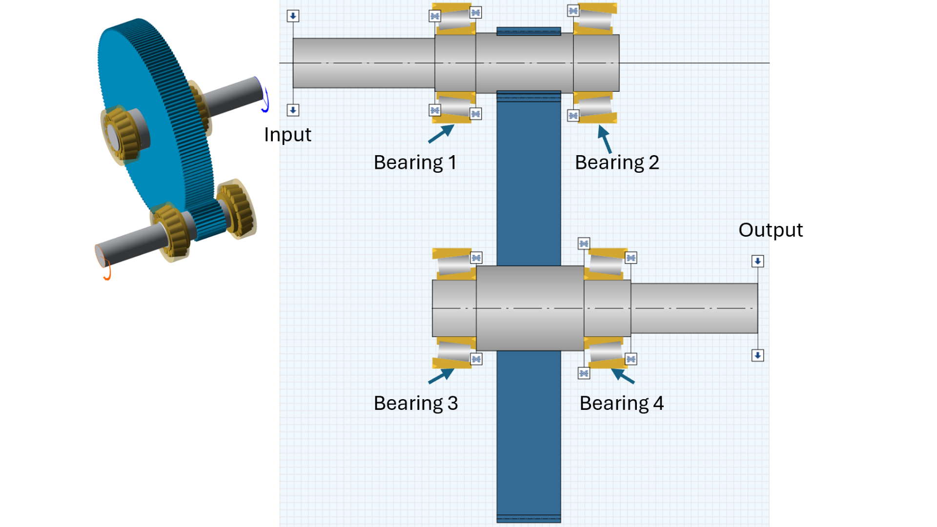
Abbildung 7: Optimiertes Mühlengetriebe
Tabelle 2: Ergebnis der berechneten Lebensdauer in Betriebsstunden für die Mühlenanwendung bei Berechnung nur mit dem Nennfall und bei Berechnung mit dem Lastkollektiv
| Modifizierte Referenzlebensdauer in Stunden unter Verwendung der nominalen Auslegung | Modifizierte Referenzlebensdauer in Stunden unter Verwendung des Lastkollektivs | |||
| ISO 281 | ISO 16281 | ISO 281 | ISO 16281 | |
| Wälzlager 1 (SKF 30216) |
1.095 | 3.435 | 1.481.170 | 2.453.468 |
| Wälzlager 2 (SKF 30216) |
706 | 1.746 | 917.652 | 1.315.214 |
| Wälzlager 3 (SKF 30216) |
2.002 | 5.108 | 1.473.792 | 2.709.666 |
| Wälzlager 4 (SKF 30216) |
2.992 | 9.691 | 2.364.789 | 5.152.745 |
Um die Lebensdauer von 100.000 Stunden unter Nennlast zu erreichen, wäre statt der Größe 30216 die Größe 32316 erforderlich. Dadurch erhöht sich die Masse der eingebauten Lager um den Faktor ≈ 4.
Abbildung 8 zeigt die Sicherheiten der kritischen Wellenkerbstellen nach der FKM-Richtlinie. Die linke Abbildung basiert auf der Berechnung mit Nennlast, die rechte Abbildung auf der Berechnung unter Verwendung des Lastkollektivs mit der Miner-Modifikation „Miner konsequent“.
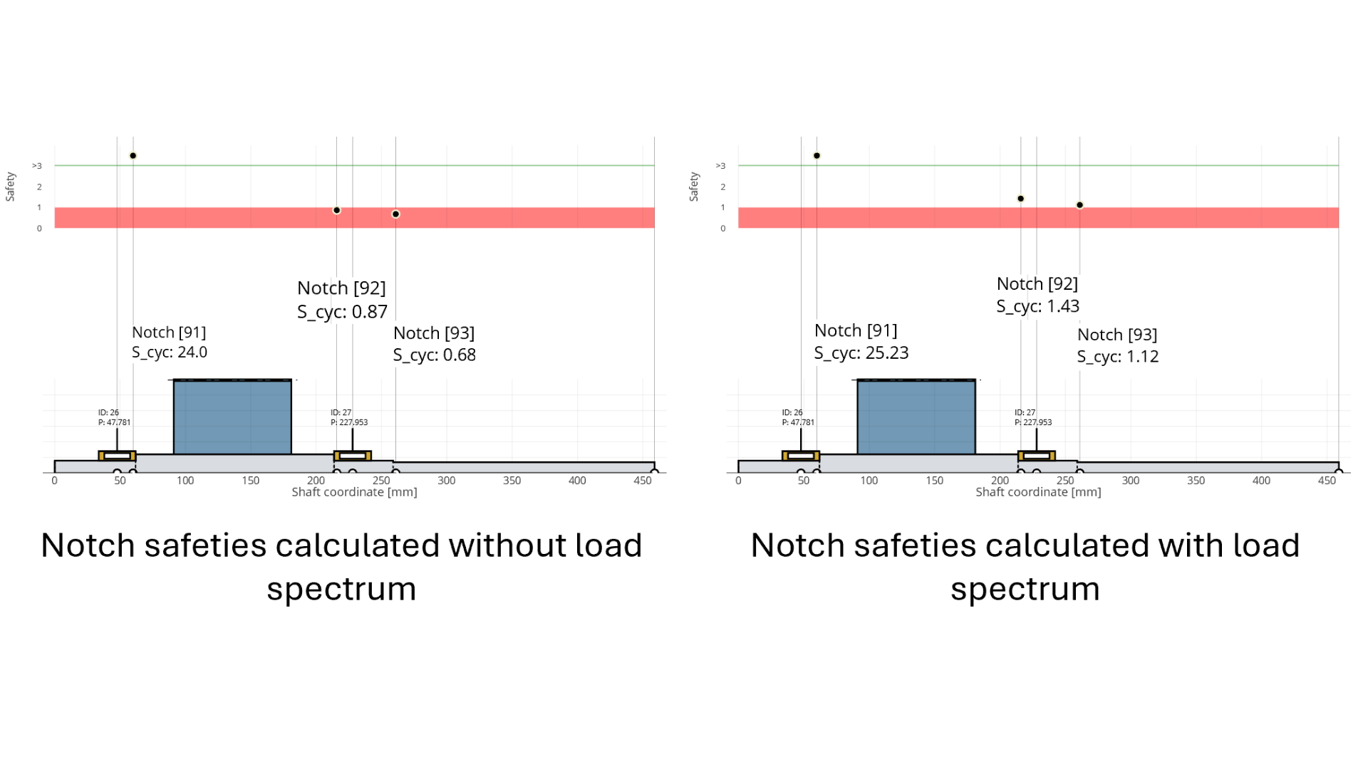
Abbildung 8: Resultierende Wellenkerbsicherheiten des optimierten Getriebekonstruktionsentwurfs
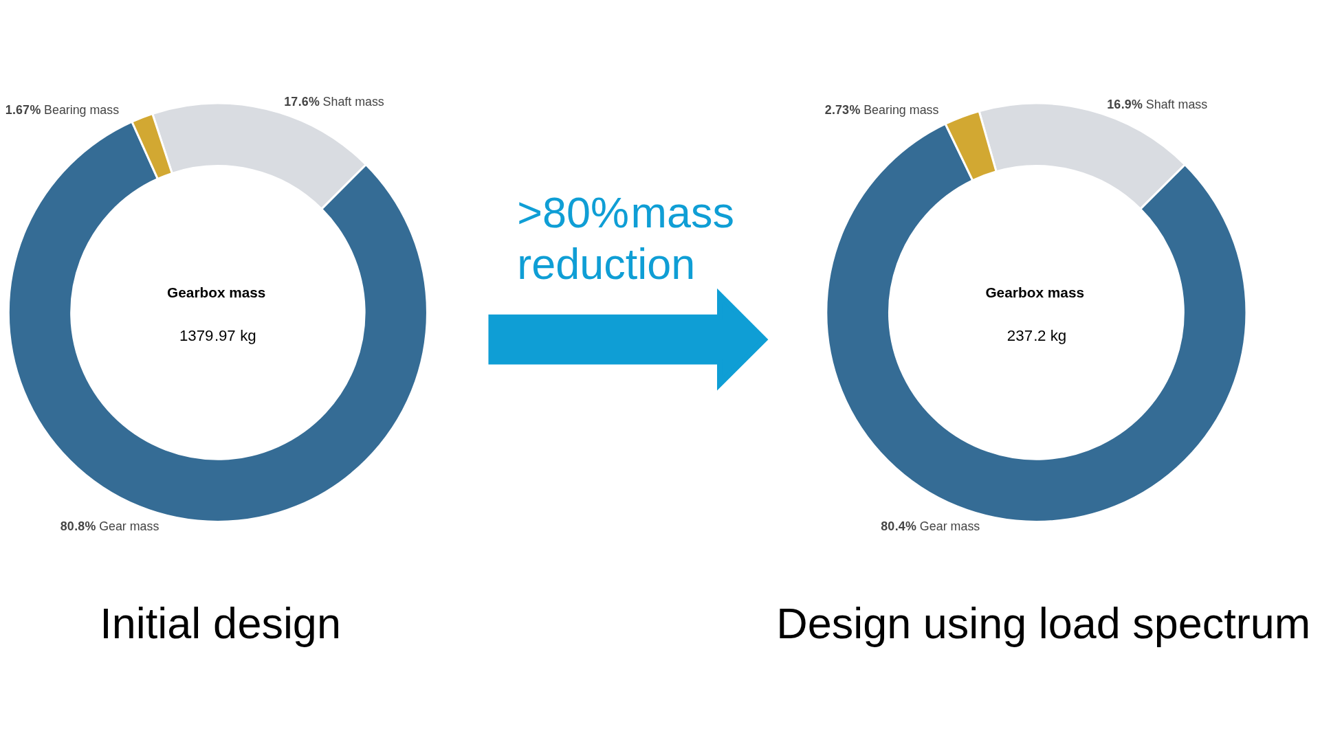
Abbildung 9: Getriebemasse vor und nach der Optimierung unter Berücksichtigung der Lastkollektive
Ohne die Berücksichtigung von Lastkollektiven wäre diese optimierte Konstruktion nicht möglich gewesen. Abbildung 9 vergleicht die Zusammensetzung der Getriebemassen bei der Konstruktion unter Nennlast und unter Verwendung des Lastkollektivs. Deutlich wird, dass die Berücksichtigung von Lastkollektiven einen erheblichen Hebel für Materialeinsparungen bietet und somit zu ressourceneffizienteren Getrieben führt.
Zusammenfassung und Ausblick
Die Berücksichtigung von Lastkollektiven ist heute ein entscheidender Faktor bei der Getriebekonstruktion, um Optimierungspotenziale auszuschöpfen und die Ressourceneffizienz deutlich zu steigern. Die FVA-Workbench bietet umfangreiche Funktionen zur Auswertung von Messsignalen, zur Erzeugung von Lastkollektiven und zur Berechnung der Tragfähigkeit auf Basis dieser Lastkollektive. Darüber hinaus unterstützt sie lastkollektivbasierte Optimierungen.
Dadurch ist die Anwendung von Lastkollektiven bei der Getriebekonstruktion mit der FVA-Workbench auch für weniger erfahrene Anwender zugänglich. So können auch Nicht-Experten das in diesem White Paper aufgezeigte Optimierungspotenzial effektiv ausschöpfen.
Referenzen
[1] ISO 281: Rolling bearings - Dynamic load ratings and rating life, 2007.
[2] ISO 16281: Rolling bearings - Methods for calculating the modified reference rating life for universally loaded rolling bearings, 2025.
[3] ISO 6336: Calculation of load capacity of spur and helical gears, 2019.
[4] ISO 10300: Calculation of load capacity of bevel gears, 2023.
[5] R. Rennert, E. Kullig, M. Vormwald, A. Esderts und M. Luke, Rechnerischer Festigkeitsnachweis für Maschinenbauteile aus Stahl, Eisenguss- und Aluminiumwerkstoffen: FKM-Richtlinie, Frankfurt am Main: VDMA Verlag, 2020.
[6] U. Clormann und T. Seeger, „Rainflow-HCM. Ein Zählverfahren für Betriebsfestigkeitsnachweise auf werkstoffmechanischer Grundlage,“ Stahlbau, Bd. 55, Nr. 3, 1986.
[7] H. D. Eisbrecher, F. W. Griese, Laumann, D. Wünsch, Kuitzsch und W. Stühler, FVA 48 I: Ermittlung und Auswertung von Lastkollektiven - Systematische, detaillierte Auswertung der Literatur zu beanspruchungsorientierten Untersuchungen an Antriebssystemen, Frankfurt am Main: Forschungsvereinigung Antriebstechnik e.V., 1976.
Autor

Dr.-Ing. Ralf Wuthenow
Head of Modeling and Simulation
FVA GmbH